Photogrammetry tutorial 13: How to handle a project in Reality Capture

Well, this is a long overdue post, and I could have saved myself a lot of emailing if I’d written it earlier. Basically, it is a sibling, even a twin to my tutorial on how to handle a project in Agisoft Metashape. Over the course of the last two years I have been using Metashape less and less, running most projects in Reality Capture. Not because it is “better” in any overall sense – both programs have their strengths and weaknesses, and I am glad to have both available. However, for my typical objects Reality Capture (RC) produces most models much faster and with a more comfortable workflow. If that fails, I typically toss my data into trusty old Metashape, which normally gives me a very good model. In a certain sense, RC is fast but princess-and-the-pea, more prone not to calculate a good alignment, and Metashape is slow but extremely robust and reliable.

One thing that also needs to be mentioned here is that RC has a very annoying bug: it will freeze and crash quite often when coloring a mesh, and sometimes also when calculating or texturing. Sometimes, re-running the project helps. Sometimes, altering the settings helps. Sometimes, removing a photo or two will help. But that means investing the time for running the model again and again and again. Therefore, I often turn to Metashape in these cases, too.

EDIT: this bug has been mostly fixed in the latest release! /Edit

So why use RC at all? As mentioned, it is faster. MUCH FASTER! So much faster that it is worth all the bother. Additionally, it has by now acquired all the little gimmicks I need, such as automated detection of coded targets.

There are several versions of RC; I here assume you use a photogrammetry capable one without Command Line Interface (CLI).

Let me begin with a quick overview of the user interface and how to adapt it to your purposes. If you are already familiar with it, you can jump down to the “Loading images” section.

When you open RC you see something like this:

I’ve marked several things here:

The blue arrow points at the quick access bar that allows altering the layout of the user interface, i.e. the number and placement of screen parts or ‘cells’ as RC calls them,

the red arrow points at the tabbed(!) application ribbon that holds all the text or icon buttons you need to work the program,

and the yellow and green circles shop the name tags of the two cells this layout offers.

 

The left cell says “1Ds” on top (yellow circle). This cell details the structure of your project – currently, all is empty. The green circle shows the name of the other cell: “3D”. Unsurprisingly, this 3D view of your project is also still empty.

During the workflow, it may be necessary to change the “1Ds” cell to previews of the images. You can do this by clicking&holding the name tag and choosing “2Ds”. Also, you will need to change the layout to one with more cells. I usually use the one that has a “1Ds” view on the left and six more cells in two rows on the right. You can switch to it by clicking the appropriate icon in the quick access bar (blue arrow). If you hover the mouse over it, a pop-up will show “1 + 2 + 2 + 2 Layout”.

You will also need to jump between the various tabs of the application ribbon. They are named on top of it: Workflow, Alignment, Reconstruction and Scene. When you click on of the words, the appropriate tab opens up – but NOT necessarily with all the icons and commands you need! What is shown depends on what cell you have active! The active cell has a blue frame around it. Just click a cell to make it active. Also, some commands are there several times, in different tabs….all a bit confusing, initially.

The RC icon at the top left of the screen is, btw, both an access to the main menu for saving and loading projects, and the exit button (if you double click it). Be warned……

 

OK, now you know all you need to know for us to proceed to

Loading Images

You can add images by either dragging&dropping them, or by importing them via the WORKFLOW tab’s “Add imagery” section. Two icons allow either adding files individually (obviously, you can select may in the explorer window) or of an entire folder.

Once images have been loaded, the “1Ds” windows changes:

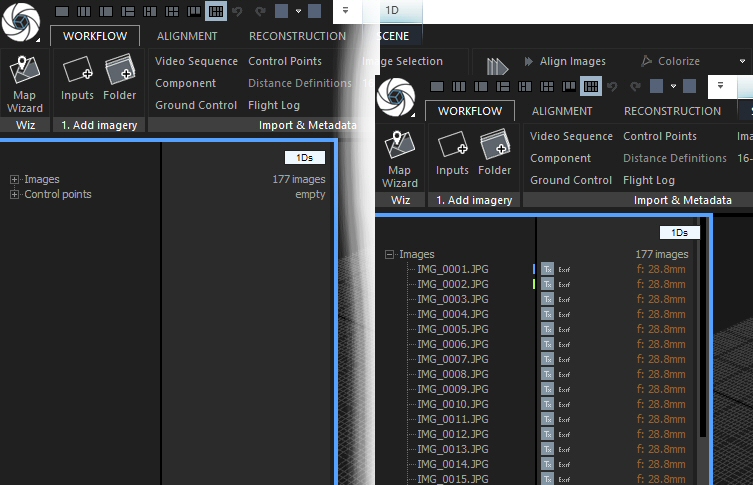
The number of loaded images is shown, and if you click the small + sign to the left of the word Images you get to see a list.

For each image, there is an icon showing if it is included in texture calculation (the grey square with Tx written on it). Click it to exclude the image. Next to it there is either text says “Exif” if there is sufficient EXIF info with the image, or nothing. And on the right the focal length is given.

You can’t remove images from a project, but you can block them from being used. Simply select them by clicking (CTRL or SHIFT to select several) and press CTRL-R to strike or re-activate them.

Now, it is time to detect markers (assuming you used coded targets) for later scaling the model. You can do without, but there is practically no reason not so use scales with coded targets these days, so I won’t get into that now. If you need scales, buy some from me: Palaeo3D Scale Bars

 

Detecting Coded Targets

Switch to the ALIGNMENT tab. In the ‘Constraints’ section, select “Detect Markers”. This opens a dialogue window at the bottom left, under the “1Ds” cell. You may have to move the boundary between them up by clicking-dragging to see the entire dialogue.

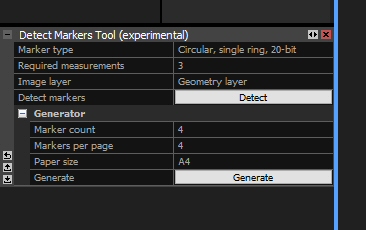
Select the appropriate type and the minimum number of images a target must be found on to be recognized (Required measurements). I’ve always used 3, which sorts out false positives quite well but recognizes targets even if a scale bar is only in a few images.

Click “Detect” and wait a short while. Now, your “1Ds” cell will look like this:

You need to click the small + to the left of “Control points” to see them. For each point, the name and number of images it is on is shown.

OK, on to….

Alignment

As you already are on the ALIGNMENT tab of the ribbon, you can simply click “Align images” in the ‘Registration’ section. Afterwards, you’ll see both a sparse point cloud in the 3D view(s) you have open, and one/a list of component(s) in the “1Ds” cell. Like this:

The upper example shows how RC creates “Components” – sets of images aligned with each other, but not aligned with any of the other images. Below, things worked  well: there is only ONE component.

If your project gets split into several components of significant size, i.e. if you feel the biggest component needs more images to give you a good model, just click “Align images” again. This will lead to fewer (ideally, one) component(s). If not, you can open the Alignment settings (click “Settings” in the ‘Registration’ section of the ALIGNMENT tab of the ribbon) and change “Merge components only” to yes to try a third time.

If all that fails, I usually abandon the project and either try by adding photos in increments or turn to Metashape.

Once you have one component that has enough images aligned, it is time for model construction.

Mesh building

RC does not give you access directly to the point cloud, as Metashape does, but builds a mesh directly.

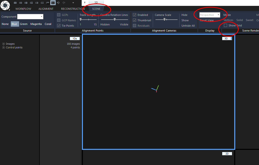
Before you start RC on building the model, you should adjust the reconstruction box – the volume that the program will work on. In the “3D” cell there should be a white box around the sparse cloud. If there is non, create one by going to the RECONSTRUCTION tab and clicking “Set Reconstruction Region”. Now, click the white outline of the box to make it editable. For easier editing, I always change the view to parallel projection and turn off the grid. You can do both in the SCENE tab, but you MUST activate the “3D” cell first by clicking into it. Otherwise, the commands you need will not be shown because they do not work in other views. Use “Show Grid” to toggle it on and off, and use the pull-down menu in the ‘Display’ section to alter the view as it fits your needs. I’ve circled the tab header and the commands in this screenshot:

Now, after you have clicked the box, it will show colored dots outside it and arrows and curves at the center. You can alter the size by  clicking&dragging the dots, and you can rotate the box by clicking&dragging on the curves. Be careful not to accidentally grab an arrow, as then you will shift the entire box happily around, which is usually unnecessary bother.

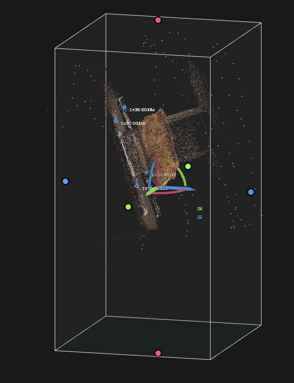
Switch back to the RECONSTRUCTION tab of the ribbon now and click “Normal Detail” all the way on the left. (Or click High detail to get a higher detail model). This will take a bit longer, and it requires an NVIDIA GPU.  The result ideally looks something like this:

Uh, well, that’s a lot of stuff all over that I don’t want or need! Notice the small bone shape in the middle, a piece of a rib? That’s what I wanted…. (well, I left the box really big to ensure I got a boatload of stuff to show you here. Now to now delete it…. – a smaller box means less junk).

You can see one important advantage of RC here: notice how the bone is free-floating? I can assure you that it didn’t float in space when I photographed it. And that I didn’t go to any extra trouble to make a special support for it that was totally translucent. No, there is ample support material in the images, which is the source for all the junk around the bone in the model – BUT the model itself is free from it! That’s because RC checks if there is “something” between the cameras and the dense part of the sparse cloud, and if there is, it won’t get built! And that makes the next task so ludicrously easy: cutting the model down to the desired object!

Model editing

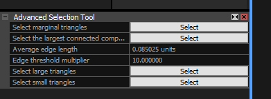
Stay on the RECONSTRUCTION tab and select “Advanced” in the ‘Selection’ section. This opens a box dialogue in the lower left, where you can click the SELECT button to the right of “Select the largest connected component”.

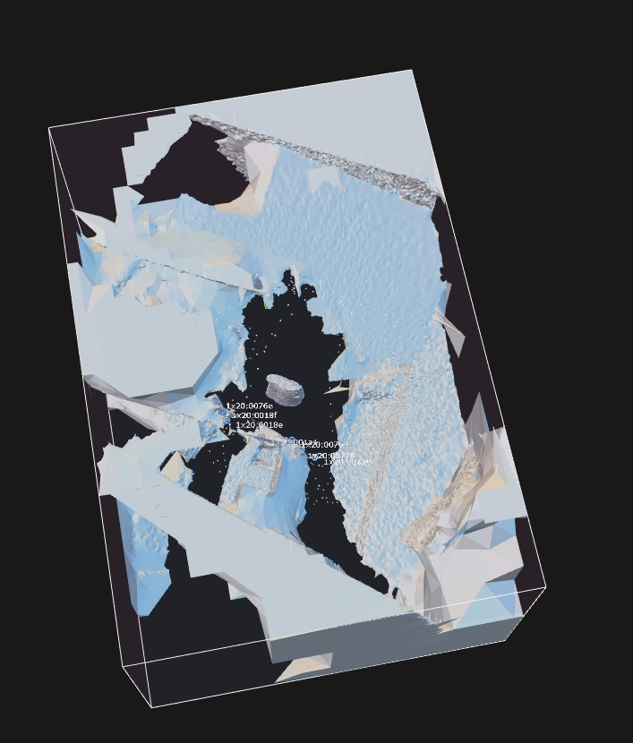
This is what you get: the largest component is highlighted in orange.

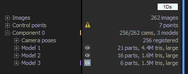
If, as is the case here, the highlighted part is NOT the desired object, click “Filter Selection” in the ‘Tools’ area. Rinse and repeat, until the highlighted bit IS the desired object, click “Invert” in the ‘Selection’ area and THEN “Filter Selection”. Now, all that is left is the object you wanted, and the “1Ds” cell looks something like this:

As you can see, RC doesn’t EDIT a model, but makes a copy and edits that. This way, you can always go back if needs be. However, it also means that the project save gets a lot bigger. Therefore, delete the old models now: if you hover the mouse just to the left of the eye icon, an X icon turns up. Click it to delete! RC will cross out the model, and after a few seconds (time to un-do an erroneous delete) it will be gone.

What are you saying? Your model is connected to some of the junk? Well, you can use the “Lasso” tool from the ‘Tools’ section to select the polygons causing the connection, and “Filter Selection” to remove them. If the resulting hole in your model is tiny, all is well. Otherwise, you can export the model now, retopologize it in some other program, and reimport it.

Next up:

Scaling

I typically use the “1 + 2 + 2 + 2” Layout for this step. Click the + next to “Constraints” in the “1Ds” cell, then click the + next to the last CP in the list.

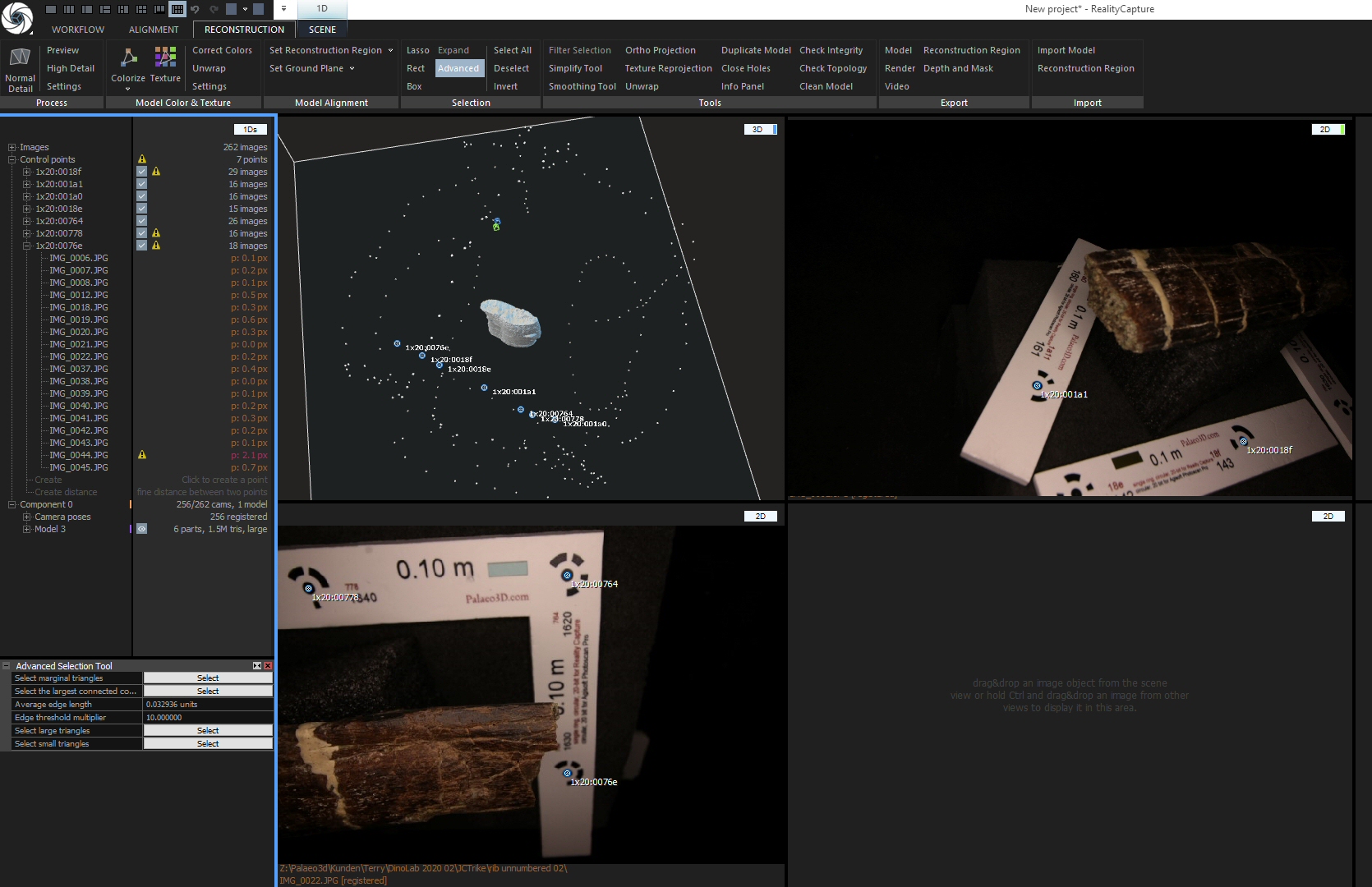
See the ugly yellow triangle? It means that one or more of the CP placements on (an) image(s) is/are bad. Could be worse than this case: there could be many, and some triangles could be red. I don’t need to tell you tha red means a bigger deviation from the average than yellow.

You can now simply delete the CP assignment from the image marked with the triangle by clicking just to the left of the triangle: an X icon will appear that deletes it. I always start with the image with the highest deviation, and work my way down, as any deletion alters the values for all other images. Once that is done, I drag&drop one image from this CP’s list into one of the “2d” cells. It will show the CP – and usually other CPs as well, which is useful – as a blue dot with its name next to it.

If the image contains a complete scale bar (as the bottom left one in the example above does), the distance can be marked right in this photo. Otherwise, open the next CP and drag a photo into another cell. Continue, until you can see both ends of a scale bar.

Now, go to the ALIGNMENT tab and select “Define distance”. Now click&hold onto the blue CP at one end of the scale bar and drag over to the CP at the other end – within one image or in several doesn’t matter. Once you let go the mouse button, a constraint is created, connecting the two CPs. Go through all the CPs in the list until all desired constraints have been created and all red and yellow triangles are gone.

Above the CPs in the “1Ds” list you can now see the created distances. The “3D” cell also shows them as lines, orange and blue (selected). Select all of the same length by holding down CTRL (CAUTION: when you use SHIFT the program may crash!). At the bottom left you now see a new dialogue window:

DEFINED DISTANCE is the distance YOU define for the constraint. RC automatically sets it at a very tiny value that is not 0, because if you were to update while it is zero, the model would be shot. CALCULATED DISTANCE is what it currently has in the program. Now, simply enter the desired length for Defined distance! This tells RC what length they should be. Now, In the ALIGNMENT TAB, click “Update” in the ‘Registration’ section. This scales the model.

NOW is the time I actually save most of my projects. Only big ones that take long to align get saved earlier, before the mesh is built.

 

Next steps: coloring and/or texturing the mesh, or decimating it…. as you please! DO save before you start, because the coloring and texturing steps are crash-prone!

Color, Texture, Decimate

Color can be found in the RECONSTRUCTION tab; it’s a big icon. Right next to it is texture. Resizing goes via the “Simplify Tool”, to be found in the ‘Tools’ part of the RECONSTRUCTION tab. It opens a dialogue at the bottom left where you set the target triangle number and click OK.

Export

Obviously, you can export a whole lot of stuff, but the key interest is certainly meshes. These can be exported both from the WORKFLOW and the RECONSTRUCTION tabs, using the “Model” command in the respective ‘Export’ sections.

 

And that, generally, is all!

There are many other aspects to working with RC, but I sure try to take my photos in a way that allows me to use this fairly straightforward and hassle-free workflow. You should, too!