EDIT June 3, 2022
Up to speed with the latest version of Metashape. Added mesh creation from depth maps.
Also see Workflow Tutorial post here!
/EDIT
Over the course of the last few year decade and more I have helped a bunch lot of people with their photogrammetry projects. Usually, they needed help with the photography – understanding how the program works, so that they take the right amounts of photographs in the right places. Or with camera settings. Or with the set-up for easy and quick models that show the underside of a specimen, too.
Recently A long time ago, however, I realized that a lot of people also have problems making the most out of their photographs in their photogrammetry software, most of them using Agisoft‘s really easy to use Metashape (previously Photoscan). They’d run through the “Workflow” menu of Metashape and end up with model that were OK or so-so, based on photographs that should deliver really excellent models.
Below, therefore, I’ll describe how I use Metashape to create high-quality models. Models like the one in this screenshot:

(click for larger size. Note that I decreased model size from ca. 45 million polygons to 10 million)
PLEASE NOTE: this post assumes that you are using Metashape Pro, not the Standard version! Some steps described below are not available in the Standard Version!
Before we get into the details of Heinrich’s Photogrammetry Work Scheme, let me list the basic steps of building a 3D mesh from photographs:
- Put photographs into software.
- Have software align photographs, including building a sparse point cloud (tie points).
- Clean up the sparse cloud, create a mesh from it, and (optional) mask your images based on this mesh.
- EITHER Have software build a dense point cloud, which may need manual cleaning.
- AND have software build a polygon mesh. Mesh may need cleaning up unless you used masks.
- OR have software build a polygon mesh directly from depth maps. Mesh may need cleaning up unless you used masks.
- If you want to, have software reduce mesh size and calculate a texture for the mesh.
At some time in between, you also need to scale your model. This can be done at any time after Step 1 (I usually do this after step 3 or at the very end), and thus I will put the info on it at the end of the post.
So, how do I do these steps?
Placing the photos in the software
First of all, chunks.
Metashape allows using several separate chunks, which you can have the software perform alignment and dense point cloud building and meshing etc. on separately, then align and possible combine them later. I do not use separate chunks if I can help it. Rather, I try to make sure that all my photos show my specimen with a totally immobile background, or one that has no features at all, across all sets of photos I take. This means, for example, that if I need to flip a specimen over to photograph the underside, I move it to a different location, so that the two background are totally different from each other. This way, the only correlating features between the first set of photographs of the upper side of the specimen) and the second set (showing the underside) are all on the specimen itself. A while ago, I began regularly using more than one, but rather three or four locations to create more sets of images. As each separate set of images needs to cover less of the specimen to provide sufficient overlap with the nest set to make a good model, more separate sets make the task of photography easier.
So, just load all images into one chunk! You can do this by using the Add Photos icon, or via the “Workflow” menu and the “Add Photos” entry. Or you can simply drag&drop images into Metashape. Note that if you drag a second set in, Metashape will create a new chunk for them, unless you explicitly drag them onto the old chunk in the Workspace list. If that happens, simply drag them from the new chunk into the old one.
And that’s it! 🙂 Step 1 completed! Unless you want or need to use masks alreadly. A huge topic of their own, which I will address elsewhere. Here’s let’s simply assume you do not need to mask anything at this stage.
Having the software align the photos
This step is not tricky at all: simply go to the “Workflow” menu and select “Align photos”. You now face a pop-up window with options:

Uh, erh….. em…. what now?
Simply stated, accuracy determines how fine-tuned the camera position determination is. For a quick check you can set it to low, but otherwise keep it on “high”.
Generic preselection basically allows the program to spend some time finding out which photo pairs likely do not overlap anyways, and can thus be skipped during later steps, which can save quite some calculation time. If you take a series of photos of a long dinosaur track, for example, there are photos from the beginning and from the end of the track that cannot show the same points ever – and thus any checking for matching points is a waste of time. I typically leave this option on “enabled”. Sometimes, tuning it off can help getting an alignment, so if a project fails try it again with generic preselection turned off. Brace for a much longer alignment time, though!
The “Advanced” section holds three very important settings.
The key point limit basically tells the program how finely it is supposed to sample each photo. Higher values mean more features (point that may be re-recognized on other photos) are to be looked for, and thus there is a higher chance such alignments will work and be of high quality. At the cost of a much longer calculation time. 100,000 is a good value for me, so try it out. Actually, there is a guy on the internet who ran exhaustive tests, and he found that values higher than 40k do little good. But sometimes, you can rescue a project by using a higher value. If you have all the computer power in the world, type a 0 into this field (which means “unlimited”).
Tie point limit sets a limit on the number of points that tie one image to another. Theoretically, 3 is the minimum you need, but the more the better. I usually keep this 0, which means “no limit”. And there is a very good reason for creating a healthy number of key points and keeping as many tie points as possible – see below wrt masking.
Then, there is a pull-down option to select how to apply the masks (if there are any). For now, let’s assume you aren’t in need of masking your images and thus have not loaded any masks. Then, the box is greyed out.
Finally, there are check-boxes offering
OPTIMIZE TIE POINT CLOUD AND ALIGNMENT
Yes indeed – a key work step that has no entry of its own in Metashape’s Workflow menu! It is, however, of paramount importance if you want to create really good models. Go to the “Model” menu and select “Gradual selection“.
Actually, before you do this, right-click your current chunk in the Workspace window and select “Duplicate chunk”, then proceed with the copy. That way, if you mess up you can simply go back to the original chunk, make a new duplicate and start over.
Ok, now open the gradual selection dialogue. A pop-up appears, offering four different options.
The first option to choose is “Reconstruction uncertainty“. When you do so, the slider will show numbers between 0 (on the right) and a varying number on the left – likely one in the middle to high hundreds. Simply click into the field and type “10“. Your computer will think for a second, and you’ll see a large bunch of points in the sparse cloud selected (turning pink). Click “OK” and delete all the selected points. You can do this by pressing the [delete] key of by clicking on the appropriate icon. If the [delete] key doesn’t work, you need to click once(!) into the model window to activate it, and press [delete] again.
And yes, delete all those points. All of them. Basically, you’re throwing out a bunch of tie points that have a low likelihood of being in the right place.
If you now check the spare point cloud again you’ll notice that all of a sudden a lot of the floating nonsense data has disappeared. If you’re lucky, you have a much clearer view of the object you were digitizing. If you are unlucky, you removed so many points that you just killed the model. If that’s the case (and you will notice this soon), it is best to start again by taking new photos. You might want to try with a higher number than 10, but usually that results in a pretty shitty model.
Next, you now need to tell Metashape to optimize the alignment of the cameras based only on the high-quality points you retained. To do this, click the little “Update” icon that looks like a wizard’s wand.

Here it is, in the middle.
If you can’t see such an icon, that’s because you can’t see the ‘reference’ pane. It’s the second tab hiding behind the ‘Workspace’ pane – you can simply select it, then drag and drop it so that it is below and not behind the other pane. In any case, go there and select the icon.
If you are using the Standard edition, you won’t fine a reference pane and wizard’s wand icon. However, you can still optimize your point cloud: go to the Tools menu, and select the “Optimize cameras” option. 😉
Metashape will now show you a window that lists a lot of parameters you can select. Simply select “Adaptive camera model fitting”. The ensuing calculations can take a few minutes. And Metashape may inform you that some cameras (photos) have too few tie points left and will be tossed out of the alignment. That’s OK, unless your photos are very bad and you should start over again anyways, so click OK.
In the end, you’ll see your sparse point cloud again, and the quality of the alignment will have improved. On to the next step: Select “Gradual Selection” again, and this time check the “Reprojection Error” option. Change it so that it is not much higher than 0.5, delete the selected points, and click that wizard’s wand icon again. Normally, though, there will not be any points with values above 0.5 to begin with. Now, click the “Update” icon again.
Next, select “Gradual Selection” again (yeah, yeah, it does get old), and this time check the “Projection Accuracy” option. I must admit that I do not really understand too much of how it works, and that I have seen very variable numbers shown for this option. However, if there are values much higher than 10, I normally enter 10 and delete the selected points. If the number of points selected is less than ca. 10% of the total, I often go down to a value of 8 or even 7, until I hit 10%. That doesn’t sound like much, but I have seen models improve quite a bit by deleting these points. Anyways, kill the points and hit you-know-which-icon.
If you wonder why I recommend you do this all, check this post. It has pictures. No, not of cats.
And finally, this step is DONE! On to the next……
Ha! Not so fast! Before we proceed, you should spend some time turning the sparse cloud around and checking it. Sometimes, you can immediately see if there are problems. A common one is that your model is there twice, with a very slight offset between the two versions. Or you can see a bunch of nonsense points, duplicating part of the object. Usually, that’s bad news and means a lot of work coming your way, but there’s nothing stopping you from trying to improve your odds and manually editing your sparse point cloud. Simply select points you do not like (usually, using the lasso tool is a good idea) and delete them, then hit you-know-which-icon again.
Now, is it time to
Pare down the spare cloud to the specimen and create masks
Note: you can skip the masks. Then, you end up with floating nonsense mesh bits or dense cloud points around your object, and if you are unlucky you may end up with mesh nonsense attached to the object. The former is no problem (see below), the latter means you should go back to this step and use masks.
So, masking….. Your sparse cloud will normally now contain a lot of points that pertain to your object, but also a lot of points pertaining to the background(s) – the table or piece of foam or whatever the object rested on during photography, as well as other stuff simply lurking and getting caught in your photos. Select the lasso tool and remove all the background. Simply circle the points and delete them. Try hard not to remove points pertaining to the object though.
If now you have Metashape build a mesh to use for masking, it will do so within the selected box – and you should make sure that the object you intend to model is fully within the selection box, and as little else as possible. So, use the icons (at the very top) for rotating and scaling the box to fit.
Now, go to the “Workflow” menu and select “Build Mesh”. You’ll see this pop-up:

Un-tick “Calculate vertex colors”, then click “OK”. Metashape will now calculate a mesh from the sparse cloud. It will probably look fairly rough, but that’s good enough for what we want to do with it: mask the photos so that only your specimen remains un-masked.
Go to the “File” menu and select “Import –> Import Masks”.

Select “From Model”, “Replacement” and “All cameras”, and you’re all set to go! Metashape will take a short (or long, depending on the number of images) while to create the masks, which you can then check by simply opening a number of photos. If your sparse cloud was good, and represents all the specimen, the masks should not cut off anything. Sometimes, very thin projections are actually masked by accident, and you will have to edit the masks in a few photos by hand. Once you’re satisfied with the masks, you’re ready for
Having the software build a dense point cloud / build a mesh from depth maps
This is really easy, as there are entries for both in the “Workflow” menu. Haha!
If you want to go the dense cloud route, simply select the option “Build Dense Cloud“. Again, Photoscan opens a little dialogue window offering options:

Options that truly speak for themselves. Low quality means just that, high means high – golly! I recommend normally using “Medium” or “High“, but it all depends on what you want to achieve.
If you expand the hidden options you can see the options for Depth Filtering. Keep this on “Aggressive” unless you have a very good reason to do otherwise (i.e., if your otherwise perfect project was suddenly missing tiny details where you needed them preserved). “Calculate point colors” stays on, unless you are certain you will need the file for 3D printing or some other use that does no require a colored model.
Now click OK and sit back for another lengthy wait……
Btw, there is a way to speed up the dense cloud creation, unless you’re dealing with a near-flat object (such as a landscape scanned from a drone): check out this post.
Next up is the ugly task of cleaning your dense point cloud, and boy can that be a bother! Or not, depending on your photography set-up and whether you used masking as suggested above or not.
In order to remove unwanted points form a dense cloud Metashape offers several tools. You can use the various selection tools from the tool bar – I usually use only the lasso tool – to select points and then either crop to the selection or delete it. Or you can use the menu “Tool”, entry “Dense Point Cloud” –> “Select Points by Mask” or “Select Points by Color”. In the former case, you get to choose which mask(s) on one of the images is used to select all point that are covered by it/them. Very helpful if your specimen doesn’t have a complex geometry. In that case it is possible that you inadvertently select parts of the specimen, so please be careful. Always make a duplicate of the chunk and work on that only. However, if you filter points by mask the mask is applied strictly, i.e. across all data! This means that a slip made during masking can kill a desired part of your model. Thus, be careful what you do!
Selecting points by color is pretty self-explanatory. Play with the various options a bit, and try the “Pick Screen Color” option. How to do this depends a lot on background and specimen color, and so on, therefore I can’t really give you detailed recommendations.
And then you’re almost done! The next step is
Having the software build a mesh
This is really easy again, as there is an entry in the “Workflow” menu again. Haha again! Select it, and Metashape will think for a moment. Then, you get a pop-up window:

Did you go the dense cloud route? Then, obviously, the “Source data” is the dense cloud. If there is no dense cloud, you need to choose “Depth maps”.
If you are modelling a near-flat surface, e.g. the surface of earth from satellite images, you can change the surface type to Height Field. Otherwise leave it on Arbitrary.
The “Quality” selection is pretty obvious: the higher the better, but the longer the calculation time.
For face count (number of polygons to create) you can choose between three suggestions or select Custom and enter a zero 0. This will give you the full size that can be created from the dense cloud. If you select one of the other settings, Metashape will use a 0 and then downsize the mesh to what you selected. You can downsize the mesh afterwards, using the Tools –> Mesh –> Decimate Mesh option (see below), so there really is not too much of a need to decimate it automatically.
The setting for “Depth filtering” is a matter of what type of object you are modeling. The stronger you set it, the more likely are you to get good surfaces, but also to lose fine projections. So, play around with it a bit.
I’d normally leave “Interpolation” on Enabled (default). And as I normally do not classify my point clouds in separate classes, there is no need to select any point class.
Simply click OK now and wait……. a…… while……. Metashape will project a short time for the job, which will grow and grow and grow. I’ve seen initial suggestions of 5 minutes after 10% completion grow to 6 hours! This problem has shrunk in the latest versions, though. Mesh generation time is back to tolerable levels. This is especially true for depth map based meshing: it is overall much faster than going through the dense cloud step and meshing the dense cloud.
In the end, you should now have a very nice high-resolution mesh. Congratulations! If instead you have a Metashare crash, make sure that in the program settings (Tools –> Preferences; then select the Advanced tab) you have de-selected “Switch to model view by default”. It keeps Metashape from changing the view to a mesh that is too big for your computer’s dinky memory.
Always(!) save your project after meshing and before changing to mesh view. ALWAYS!
You can check the size of the mesh before you change view, too, by clicking on the + sign next to the chunk in the “Workspace” tab. It’ll show you a little triangle icon with the text “3D model”, and give the number of faces. Learn which sizes your computer can display!
If anything is too large to show, either right-click the triangle icon and export the mesh to work on it in another program. Or, resize the mesh to a more palatable size.
Whether you used masks or not, you may now have some floating nonsense parts around your object mesh. You can use “Gradual selection” (in the “Model” menu), “Connected component size” to select the stuff you don’t need. Simply delete it.
Reducing mesh size and texturing meshes
Before you downsize your mesh, I recommend duplicating it. Simply right-click the Mesh entry in the Workflow pane and choose “Duplicate Mesh”. Now, there will be two meshes in the chunk, one of them set to “active”. You can use the ” Tools –> Mesh –> Decimate Mesh” option to reduce the mesh to something palatable. I recommend against doing away with the full-size mesh if you’re planning on doing science with your data. Simply keep it in there. The display will show the “active” mesh, so make the reduced version “active” by right-clicking on its entry on the Workflow pane and selecting the appropriate entry.
In order to build a texture, simply make sure you have the correct mesh selected, then go to the “Workflow” menu and select “Build Texture”.
OK, that’s all! Have fun 🙂 And if you still have any questions or problems, email me or ask for help in the comments here!
Scaling your model
As I mentioned above, you can scale your model at various stages of the process. I typically scale as late as possible, simply because a model may fail for various reasons during the process. Scaling is a not a lot of effort, but it is effort, and if a model fails fatally, then that work is wasted. On the other hand, I have had cases where I forgot to scale and ended up using 3D data that was un-scaled. Luckily, I or someone else always noticed in time – e.g. before a 3D print was started and monetary costs ensued. But it may still be a good idea to scale early in the process, always at the same step of the process, just to make sure that you never use un-scaled data by accident.
In order to scale a Metashape project you need an object of known size in your photos. Obviously, the easier way to achieve this is placing a good old scale bar next to specimen during photography. Or, better, several scale bars. If you’re a lazy fuck (like me), there are so-called ‘coded targets’ – scale symbols Metashape can recognize automatically. More on that below. Let’s begin this with the hard-core way of scaling.
Metashape can scale a model only if there is a in-program scale bar. Such a scale bar can be created from two in-program markers, which in turn need to be identified by you on at least two photographs. That’s easily done: In the (empty) marker list in the Reference pane, right-click and select ‘Add Marker’ or use the icon to create a marker. That’s the only way of creating a new marker that Metashape won’t project all over the images, and we don’t want it projected. Now, right-click the marker and choose ‘Rename Marker’.
It doesn’t really matter what name you give the marker, just make sure that it makes sense to you. You can even stick with the default name, but I find it helpful to give ‘speaking’ names. If, for example, you have a scale with numbers, I’d name the makers ‘0 cm’ or ‘2 cm’ or ’10 cm’, depending on where you place them. That way, it is easier to pick markers from a list and immediately know how long the scale bar between them is in reality, and thus should be made in Metashape.
Now, select a photo and open it by double-clicking. Right-click on the place the marker is supposed to go, and choose ‘Place Marker’ and then the marker you wish to place from the list.
If you place markers after aligning the photos, when you’ve placed a marker in one photo, Metashape will put a line onto other photos showing where it projects the marker to. In essence, it shows you the trace of the position vector from the previous camera position through the marker on all other cameras that look the right way. Whether you aligned the photo already or not, now all you need to do is to repeat the above-described process: right-click the image in the correct location (which in the case of a sub-optimal alignment may be off the displayed line), select ‘Place Marker’, and choose the appropriate marker name. If you ran alignment before, you now basically gave Metashape two place vectors from two positions the relative alignment of which is known – and the marker must thus be located in the place the two vectors intersect! Hurrah!
Next, you simply select the two markers that describe your real-life scale bar and create an in-program scale-bar. Selection is easy: click one in the list in the ‘Reference’ tab, press and hold [CTRL], and select the other. Then, right-click and select ‘Create Scale Bar’. DONE!
Now, the bottom-most part of the ‘Reference’ tab will show a scale bar. You now need to assign a length to it (simply click the correct line in the “Distance” column and enter the correct distance; remember this is in meters!). Do this for all the scale bars you created (more than one is a good idea!), then click the ‘Update’ icon in the ‘Reference’ tab. It shows two arrows going opposite ways and is next to the you-know-what ‘Optimize Cameras’ icon. Here’s that screenshot from above again, which shows you what the icon looks like. It’s to the right of the Wizard’s wand icon.
AND DONE!
Yes, it really just takes a split-second and your model has been scaled. Check out the “Error” column in the ‘Reference’ tab (you may need to move the scroll bar to the right. If you did good on, say, a sauropod bone, you’ll see 4 decimal zeros 🙂
Coded targets
In Metashape you can print out circles with black and white patterns. They all have a little white dot in the center. If these are in your photographs, you can ask Metashape to go looking for them and automatically assign markers to them. If all goes well, you just saved a lot of marker placing, and only need to create the appropriate scale bars. However, before you can do all this, you need to create real-life scales with two coded targets each, print them out, and place them next to your specimens. My colleague Matteo has done this, and we have been using these scales with mixed success. It turns out that the coded targets, nice and large on our scales, are too big to be found by Metashape if we take close-up shots of bones. In the field, where the photos typically show larger areas and the coded targets are proportionally smaller on the images, they work flawlessly.
Later, I started making my own scale bars with coded targets, and by now I must say they are pretty good! I’m selling them at quite affordable prices via my company website: http://palaeo3d.de/WP/?page_id=23
In order to trigger a search for coded targets, choose “Markers” –> “Detect Markers” in the “Tools” menu. Select the type of targets you used in the photos, and click “OK”. If you know that only a certain range of your photos in the project includes markers, you can select them before you start the command, and use the tick box “Restrict to selected images”. That’s obviously quite a bit faster 🙂
Now go and have fun with easy-peasy scaling!

Pingback: Photogrammetry tutorial add-on: The consequences of optimizing a sparse point cloud | dinosaurpalaeo
Pingback: PaleoNews #18 (National Fossil Day 2015 Special Edition) | An Odyssey of Time
Thank you for the nice tutorial. Can you explain the meaning of the 10 at the point “Reconstruction uncertainty“, please?
Thomas, that’s just a value I found to work well! If you choose too low a value (say, 4), you delete too many points. If you leave the value too high, you retain too many bad points.
As I said, I do not know exactly what the various parameters do. Agisoft doesn’t explain this in detail in their manuals. All I found is this:
“High reconstruction uncertainty is typical for points, reconstructed from nearby photos with small baseline. Such points can noticably deviate from the object surface, introducing noise in the point cloud. While removal of such points should not affect the accuracy of optimization, it may be useful to remove them before building geometry in Point Cloud mode or for better visual appearence of the point cloud.”
whoa!
nice tutorial dood 😀
extra information will definitely come handy
cheers
Great Turtorial, Thanks.
Can you advise when would be the best part of the process to add in Ground Control Points for Aerial work?
Thanks so much.
sorry, I can’t make any recommendations on this, as I have exactly zero experience with aerial data. But I guess it doesn’t hurt to add them early in the process.
Thank you for your response Heinrich. Your tutorial has been very helpful nonetheless!
Thank you for taking the time to write it.
glad you like it 🙂
Really complete and nice tutorial! thanks for sharing all that wonderful experience with as many details and reasons to understand a little more how the software works.
Just one question, about the tie points cleaning (thanks so much to talk about it, is the first time i read this process and yes this solve many problems in some models I have done) Can you explain how to do it properly in the version 1.1.6?
Thanks!
it has pass 4 years and this link still the holly grail reference to work with photoscann or now metashape
I know right! I turned my adblocker off on this site just as a way of gratitude so Heinrich can get some return for his effort!
ha! Thank you – I get nothing but continued free hosting, but that’s something at least.
However, it seems that everyone now gets ads, so maybe it is time for me to upgrade.
Thank you!
I guess this needs an update, though: Metashape has improved quite a bit since the last installment.
This tutorial is a little nugget of gold – thanks 🙂
Thank you for your article, it was great help, especially the part about point cloud and image alignment optimization!
What I was wondering about was how large the dense point cloud usually get for you? How many points?
I myself regularly work with archaeological data with Photogrammetry, but mostly with excavation data, which is quite different from what you are working here. Where you have to capture the fine details of a given object, an excavation trench is too large for such a level of detail (and in most cases doesn’t even need that much detail), and would require too much computing, not to mention the amount of photographs needed. With these differences in mind it will be interesting to see if (and where) the settings and the tresholds you used will need to be changed for such a different application. I’ll make sure to document it. 🙂
Bence,
the size of the dense cloud really depends on the circumstances. Anything between 500.000 and 3.5 billion is on 😉
For a large sauropod bone I would aim for some 1.5 million points, but the finished mesh will usually get downsized to ca. 150.000 polygons anyways.
As for excavations – these are similar to tracksites, which I have done. The same problem for both: you need high-res in specific locations that you can’t afford to produce overall. I usually solve this by making a low-res model from photos able to provide high-res, then duplicating the chunk over and over again, and making in each chunk a high-res model of the details. These I copy into the overview model after cropping them to the object I really want.
You mention the first time the sparse cloud is optimized with the gradual selection process that if using the Standard Edition, one can choose “Optimize cameras” instead of the (missing) Wizard’s wand icon. With Standard Edition, does choosing “Optimize cameras” instead of the wand icon work for each of the additional gradual selection steps?
Thank you for a well written tutorial.
Lawrence,
yes, you can always access this command via the menu!
can you give the dimensions of your scale with coded targets?
they vary, depending on specimen size. I have 10 cm, 15 cm, 20 cm, 25 cm, 50 cm.
Thank you so much for this tutorial. I just have a question about scaling…Is this necessarry? I have made a 3d model of a small object that I want to scale up, with 3d printing, so the original size doesn’t really matter.
Well, if you have a certain fixed size in mind that you wish to scale your object to, then it is not necessary.
Pingback: The Basic PhotoScan Process – Step 4 – Public Archaeology in 3D
Hi Heinrich,
this is to let you know that I appreciate all the effort you put into this tutorial. It totally made the difference! I only use the standard edition but your article made quite a difference. So agian, thanks.
Cheers!
Great…but what if you do need to mask backgrounds? What is the best approach?
Iain, there are many approaches. Hard-core manual masking in Photoscan, importing a mask based on the background (you take a photo of your turntable without the specimen on it, which then gets used to mask your images where they do not differ), masking based on alpha channel, etc. It is a huge topic to cover, and I simply haven’t gotten around to it.
Hi, thanks for the info.
Can you tell me some values of reference for the spare cloud, dense cloud and mesh?
I’m trying to rebuild a human head, and I’ve get differents results.
Sometimes, the alignment end with 5k-6k points, and sometimes with 35k points… Is there a minimun of necessary numbers of points to continue?
well, the number of points that you should reasonably have depends on the number of images you use and their resolution. 100 images at 24 MP each should see sparse cloud points in the range of, say, 50k to 300k, depending on overlap etc. You have to develop a feel for it, and the sheer number of points doesn’t really matter.
thank you
Hey, great tutorial I’ve been using the optimizing tricks on most projects now.
I did a test for research and curiosity purposes, comparing the time taken for dense cloud generating of an non-optimized point cloud vs optimized point cloud, there was not a lot of difference in time taken.
Do you have any other tricks to decrease the processing time?
Or is this something that is just going to take time without having to look at improving computer hardware?
The time for dense cloud creation should remain roughly the same, unless you kick out a lot of images when optimizing.
To make things faster: Make sure your box includes only the bits you really want to model! Also, remember that you can make the box SMALLER, which reconstructs only a part, duplicate the chunk, set another box, and reconstruct that area, then combine the two chunks (after[!] aligning them based on cameras). Sometimes, with extreme geometries, this is indeed faster than having one huge box that reconstucts a lot of background.
Do use the generic preselection for matching. It rarely hurts, and speeds things up a lot.
check in the latest version you have GPU calculation option, but you need to activated it. unlikely I think it’s only for the first step.
Pingback: Photogrammetry tutorial 11: How to handle a project in Agisoft Photoscan | Aedificium
Thank you for this helpful tutorial! I usually take 3D scans of food and always have trouble capturing the bottom of the plate. After reading this post, I’m curious to know if you would suggest taking the same plate as the one the dish is on, inverting it onto a different surface (i.e. a black tablecloth instead of a white tablecloth, which is what I usually shoot on) and taking photos of the bottom of the plate, then combining the photos together in AgiSoft to align?
Pingback: Photogrammetry: index to Heinrich Mallison’s tutorials | Sauropod Vertebra Picture of the Week
This is an excellent guide. Thanks for sharing the post.
Pingback: Photogrammetry tutorial 12: my workflow for Agisoft Photoscan as a diagram | dinosaurpalaeo
Thank you so much for writing such a detailed and informative guide through your posts and your excellent paper. I’m new to photogrammetry and am learning it before using it extensively as part of my PhD and your guides have taught me so much so far!
Thanks for this! I have a cloud created model i’m trying to match the detail from using Metshape and it’s showing me just how much there is to consider… It’s not just a “import > Process > yey!” job.
Pingback: Photogrammetry tutorial 13: How to handle a project in Reality Capture | dinosaurpalaeo
Hi Heinrich,
Thanks for putting together your workflow for those of us who have less experience than you.
I am working on a fossil skull and I have six sets of photographs: Three sets (36 photos each shot on a turntable at 10° increments) of the dorsal side (one set at 80°, one at 60°, and one set at 30° angles projecting downward). Also I have three more sets where the skull was inverted, now ventral side up, and using the same angles as for the dorsal side. This provides 216 images in total.
First I loaded the 108 dorsal images into one chunk (I’m using Metashape 1.6 standard) and ran Align Photos using Moderate accuracy, 100,000 Key point limit, 0 Tie point limit, apply masks to Tie points (I’ve masked every alternate photo), and Adaptive camera model fitting. When I run Align Photos under these conditions the resulting sparse cloud shows the dorsal view nicely. (I will rerun this later at High accuracy but just now my goal is to get my methods worked out.) I repeated this test using just the three sets of ventral views and again got a nice sparse cloud. Thus encouraged I placed all 216 photos in one chunk and realigned them (being sure to click the Reset current alignment box) but I only see the dorsal side of the skull.
Next I added a set of straight lateral views thinking that this might provide an extra “bridge” to connect the dorsal and ventral views. When I add these images into the chunk, now 252 photos, I get the dorsal and ventral views superimposed; canines projecting in both directions! An interesting skull but not a happy outcome.
I would be most appreciative of any guidance you can give me.
Danke,
Stuart White
Cool, very cool.
Specialy, because is so detailled. And quite written with humour. 🙂
I had hoped, that at least the step with “texture” and its option – box would also be explained deeper, but I cannot find this.
But maybe this is simply not that important, I have choosen the defaults.
Thanks for your work!
Thank you so much for this set of tutorials. I have called attention to these many times – they are so spot on and great at expressing what one needs to be able to create models with Metashape. I appreciate your hard work here, so much! (Paleogirl on Sketchfab)
If I had used a print version of this it would be see-through by now; I’ve used it or referred others to it so many times. Thank you for this excellent guide!
Thank you! I try to keep this up to date, but sometimes there are just too many changes.
Heinrich, just wanted to drop a sincere thank you for this article and, especially, the continued updates over the years. It is a reliable reference for me. Cheers!
Grant, many thanks for the praise!
Pingback: A revival? | dinosaurpalaeo
I tried to follow your instructions. The dense mesh cloud turned out very smooth and detailed. But the 3D model is rough and inaccurate. Building mesh process was at option “high”. What am I doing wrong? Thank you.
Dmitrii, did you check that you are building the mesh from the dense cloud?
I think I understand the problem. In your manual, the face count option in the build mesh menu is set to zero. This makes the 3D model very low polygonal. I set the value to “high 180000”. The model now has a very smooth surface.
Going back to your tutorials again and again. Is there an option in metashape and any instructions on your site to fix the masks. Thank you.